
1. Introduction
Landscape judgments depend on the conditions under which places become available to perception. Drawings, photographs, moving images and recorded sound each preserve certain relationships while withholding others. A recording may make a distant environment audible in a consultation room, yet it also fixes a listening position, selects a duration and translates a spatial encounter into a particular playback arrangement. These decisions matter when participants compare places through the material presented to them. Agreement between the average scores obtained with two arrangements does not necessarily establish that individual participants encounter the same comparative relationships. The issue is whether a representation preserves the judgment required for its intended use.
Sensory approaches to landscape architecture place listening within a broader account of movement, atmosphere and embodied experience [1]. Sound introduces temporal events that cannot be read directly from a plan: approaching traffic, intermittent conversation, water movement or changes in activity. Such events can help communicate a place, but their audibility does not establish their desirability. A convincing recording of an intrusive environment may create strong presence while offering little comfort. The distinction between communicating a place and evaluating its quality therefore requires explicit treatment. Without it, technical claims about audio presentation can become unsupported claims about landscape value.
Representations also structure what can be discussed in participatory design [2]. Their apparent immediacy can obscure the decisions that produced them, including which experiences were selected and which were omitted. The aesthetics of digital representation raise related questions about realism and abstraction [3]. For auditory material, realism cannot be reduced to the number of channels or the description of a recording as spatial. Microphone placement, spectral characteristics and reproduction conditions influence the available spatial cues [4]. Spatial audio in virtual environments consequently involves technical and perceptual choices that deserve evaluation for the particular task being undertaken [5].
A direct comparison of stereo and binaural presence already exists [6]. The present contribution does not claim priority for comparing these formats. It asks a different analytical question: whether an unchanged ordering of average presence scores conceals reversals in the comparisons made by individual listeners. This distinction connects to quantitative soundscape work that treats the distribution of responses as part of the description of a place [7]. An average can summarize a group without describing its internal agreement. When the same people assess several settings, their repeated observations permit that agreement to be examined directly rather than inferred from separate summaries.
Auditory presence refers here to the subjective experience of being situated in the represented environment. Its questionnaire tradition concerns experienced location and reality rather than environmental preference [8, 9]. Presence is neither a sound-pressure measurement nor an assessment of ecological condition. It also differs from affective dimensions used to describe soundscape quality. Research on soundscape descriptors and assessment protocols emphasizes the need to connect each measure to its intended construct [10, 11]. A presence score can therefore answer a question about the conveyed experience while leaving pleasantness, appropriateness and restoration unmeasured.
This distinction becomes especially consequential when natural and urban recordings are compared. Evidence concerning the health benefits of natural sounds addresses outcomes and exposure conditions that differ from a short presence questionnaire [12, 13]. Likewise, psychological and physiological responses to sound should not be treated as interchangeable indicators [14]. A high presence rating for traffic cannot establish harm, and a lower rating for a park cannot establish a lack of restorative potential. The present analysis retains the identity of the four recordings but confines interpretation to the answers actually collected.
Laboratory listening offers control over presentation, but correspondence with an encounter in place remains a separate empirical question. Comparisons between photographs and on-site observations demonstrate why representational validity must be evaluated rather than presumed [15]. Recent investigations of virtual and real sound environments address the same issue through different combinations of audio, vision and interaction [16, 17]. A review of ecological validity across landscape and soundscape experiments further distinguishes the factors governing transfer between laboratory and field [18]. None of those results makes an eyes-closed headphone presentation equivalent to walking through the recorded setting.
The methodological problem has two parts. One concerns sampling: repeated observations from the same person do not create additional independent participants. The other concerns measurement: ordered response categories do not automatically have equal psychological distances. Evidence from urban soundscape questionnaires gives a specific reason to examine the latter assumption [19]. More general work on ordinal responses shows that conclusions may depend on the model used to represent category spacing [20]. Accordingly, the analysis combines a transparent arithmetic score with item-level, median and threshold checks, keeping their different interpretations visible.
A further difficulty arises from the meaning of a reversal. Two nearly equal scores can cross with a very small change, whereas a reversal involving substantial contrasts in both presentations represents a larger observed disagreement. Neither pattern identifies its cause. Repeated presentations within the same format would be needed to estimate ordinary response fluctuation under otherwise similar conditions. Without that comparison, the frequency of cross-format reversals describes the observations but cannot quantify how many were caused by recording format. The distinction protects a useful descriptive result from an unsupported technological explanation.
The disciplinary distinction is narrower than a claim that sound or representation has been neglected. Existing landscape research examines sensory encounter, participation and the visual conventions through which projects become intelligible. The present question concerns a particular property of repeated auditory judgments: whether their comparative direction persists for the same listener.
The investigation examines three connected questions in thirty listeners’ assessments of four recorded settings. It estimates the average paired difference between binaural and stereo presence scores, counts the preservation and reversal of within-listener setting comparisons, and examines dependence on missing answers, score construction and presentation position. Its contribution to landscape architecture lies in connecting the level of analytical agreement to the intended use of auditory representation. The four recordings are treated as fixed examples rather than independent samples of entire landscape types. The resulting evidence is relevant to how recorded experiences are compared, while providing no direct test of design preference or collective decision quality.
2. Listening Observations and Analytical Procedure
2.1. Participants, recordings and observation structure
A listening experiment examined perceived presence across environmental recordings presented in stereo and binaural formats [21, 22]. Thirty participants aged 18–27 years took part (mean 21.9, SD 2.31), including sixteen female and fourteen male listeners. The present study examines their questionnaire responses to assess how reported presence varies across listening conditions and their position in the experimental sequence.
The recordings represented La Estanzuela Ecological Park, Santa Lucía Riverwalk, traffic along Eugenio Garza Sada Avenue, and the Metapatio music venue in Nuevo León, Mexico. Presenting each environment in both reproduction formats produced eight conditions per participant. The protocol included a sixty-second resting period followed by two minutes of listening and questionnaire completion. Participants listened through AKG K240 headphones with their eyes closed. Recordings were prepared at 48 kHz with 24-bit resolution, with microphone-response matching and inter-channel gain adjustment.
The analysis is confined to questionnaire responses and listening order. Audio waveforms and electroencephalographic signals were not processed, and participant-specific headphone sound-pressure levels were unavailable for adjustment. The findings therefore concern reported presence under the experimental listening conditions. They do not establish acoustic-level effects, spatial-localization accuracy, or relationships with neural activity.
After each condition, participants answered three items on a scale from one to seven, yielding 720 responses across 240 listening instances. The items assessed feeling situated within the represented environment, experiencing it as the dominant reality, and remembering the encounter as a place. Higher scores indicated a stronger sense of presence. All items were scored in the same direction and interpreted as measures of presence rather than preference.
The hierarchy was retained at each stage: answers belonged to presentations, presentations belonged to listeners, and the four settings recurred within each listener. This structure determines the unit of independent replication. Treating every answer, format pair or setting comparison as an independent person would overstate the information available. The general distinction between an observational unit and repeated measurements is well established [23]. Here, thirty participants support exploratory estimates for these fixed recordings, with limited precision and no justification for broad demographic subgroup comparisons.
2.2. Response checks and score definition
The questionnaire, demographic and presentation-order records were joined through participant and recording identifiers. Checks required a unique participant–recording–item combination, three distinct item labels for each presentation, numeric values within the permitted response range, and one presentation position for each participant–recording combination. Non-numeric dash entries were treated as absent answers. They were never assigned zero or interpreted as a neutral response. An independent calculation using integer sums confirmed the principal agreement counts and the setting-specific average differences.
For the score, all three answers had to be present. Let \(y_{isfq}\) denote the response from listener \(i\) for setting \(s\), format \(f\) and item \(q\). Presence was summarized as
where \(B\) denotes binaural and \(S\) stereo. Scores and differences are expressed in response-scale points. The arithmetic mean gives equal numerical weight to each item and assumes approximately equal distances between adjacent categories. It is used as a descriptive score, not as evidence that a new psychometric instrument has been validated.
For each setting, stereo and binaural means were calculated from exactly the same complete matched listeners. This prevents a difference from arising solely because the two means describe different people. A participant could contribute to one setting’s estimate while being excluded from another if an answer was absent. The principal analysis therefore retains available information without requiring every listener to have a complete response record for all eight presentations. A separate restriction to fully observed listeners examines the consequences of using one common sample throughout.
The validation checks addressed internal consistency of the observation structure rather than clinical or psychometric validity. A permitted integer can still reflect misunderstanding, and a complete presentation can still contain an uncertain judgment. Conversely, an absent answer need not indicate low presence. No record justified removing a numerically unusual listener as an outlier, so every participant remained eligible under the same completeness rules. This avoids a selective exclusion that could alter both average differences and reversal counts. The item-level check retained all available matched answers for that item, which explains why its denominators can exceed those of the three-item composite.
The small overall proportion of missing answer cells does not by itself establish negligible missingness bias. The effect of missing information depends on which comparisons it prevents and why the answers are absent [24]. No reason for an absent answer was available. Neither a missing-at-random assumption nor a particular imputation model could be supported from these records alone. Complete-presentation scoring was therefore paired with explicit coverage counts, a less restrictive item rule and a descriptive bound on unavailable comparisons.
2.3. Within-listener comparison outcomes
For each pair of settings \((s,t)\), the contrast within a format was
The six possible setting pairs were evaluated separately for each listener. A retained comparison required \(c_{istB}c_{istS}>0\), and a reversal required \(c_{istB}c_{istS}<0\). A zero contrast in either format was assigned to the tie category. Thus, ties include a strict distinction in one format and equality in the other, as well as equality in both. A comparison was unavailable whenever one of its four required presentation scores was absent.
Integer item sums determined the signs and equality checks. Dividing those sums by three only afterward avoided numerical round-off being mistaken for a strict ordering. This matters because the score has discrete one-third-point increments: a tiny floating-point remainder must not convert equality into a reversal. The procedure retains the difference between an observed absence of distinction and an unavailable observation. The former enters the main denominator; the latter does not.
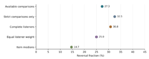
Two reversal fractions answer different questions. The principal fraction divides reversals by all available comparisons, including ties. A second fraction excludes ties and asks how often strict orderings disagree when both formats distinguish the settings. Neither denominator is inherently preferable for every design task. The inclusive denominator describes the entire set of usable comparisons; the strict denominator concentrates on decisions that actually distinguish the settings in both presentations. The confidence calculations retain listener records during resampling, consistent with the dependence structure required for clustered observations [25]. Their joint presentation prevents apparent precision from hiding the role of equal scores.
Magnitude was examined through the smaller absolute contrast across the two formats. For a reversed comparison this quantity was
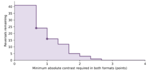
Counts above successive thresholds describe whether reversals persist when both contrasts must be appreciable on the observed scale. Two-thirds and one point were selected as transparent descriptive thresholds. They do not represent established minimum important differences, and no connection to a consequential planning choice has been validated.
2.4. Uncertainty, weighting and incomplete comparisons
Confidence intervals were obtained by drawing thirty listeners with replacement and retaining each selected listener’s entire response record. The procedure used 30,000 resamples and percentile limits at 2.5 and 97.5 percent. The random seed was 20261031. Resampling listeners rather than individual comparisons preserves the dependence among the six comparisons generated by one person. The intervals describe sampling uncertainty conditional on the observed participant pool and fixed recordings; they do not account for selection bias or variation among unobserved sites.
The main pooled reversal fraction gives each available comparison equal weight. A fully observed listener consequently contributes six comparisons, whereas a listener missing one complete presentation contributes three. To examine that weighting, an additional descriptive estimate first calculated each listener’s reversal fraction and then averaged those fractions equally across people. This estimate changes the target quantity from the fraction among available comparisons to the average listener-specific fraction. Their difference can indicate concentration of reversals among participants with more complete records without establishing the mechanism behind that concentration.
There were thirty unavailable comparisons among the 180 possible. An arithmetic bound assigns none or all of those comparisons to reversal while leaving the observed counts unchanged. It is intentionally conservative and contains no probability model for missing answers. Its purpose is to show the range compatible with complete ignorance about unavailable outcomes. Such a bound should not be interpreted as a confidence interval or as evidence that the extremes are equally plausible.
2.5. Alternative scoring and presentation position
Sensitivity checks calculated means from presentations with at least two observed answers, treated each item separately, replaced the three-item mean with its median, and counted the fraction of answers in categories six or seven. The last outcome measures upper-category occupancy and is expressed as a percentage-point difference. Its interpretation differs from a mean-score difference, even when both are calculated from the same matched presentations. Median scoring retains response order while creating fewer distinct score values, making changes in tie frequency particularly important.
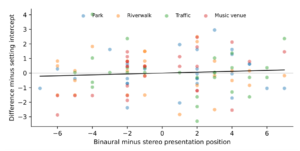
Presentation order was represented by the binaural-minus-stereo difference in presentation position. The fitted model was
with one intercept per setting and a common linear position coefficient. Ordinary least squares supplied the estimates, and 10,000 listener-level resamples supplied percentile intervals. Equal-position intercepts are model-based adjustments rather than directly observed simultaneous presentations. The adjustment does not isolate nonlinear fatigue, memory of a particular preceding recording, or carryover associated with its content.
Exact two-sided sign tests compared positive and negative nonzero differences within settings, followed by Holm adjustment across four tests. These checks concern direction, whereas the mean differences weight magnitude. Confidence intervals and graphical distributions therefore remain the principal summaries. Failure to reject a null hypothesis does not establish equivalence; that would require a justified tolerance and an analysis designed for that purpose [26]. The emphasis on estimates and their uncertainty follows broader arguments for interpreting quantitative evidence beyond thresholded significance [27, 28].
3. Results
3.1. Coverage and the distribution of presence responses
Fifteen answer cells were absent, accounting for 2.1% of the complete response structure. They affected ten presentations belonging to ten different listeners, leaving 230 complete presentations. The matched format comparisons numbered 27 for the ecological park, 28 for the riverwalk, 28 for traffic and 27 for the music venue. The coverage display in Figure 1 locates the incomplete presentations within the repeated listening structure. The setting codes are P for park, R for riverwalk, T for traffic and M for music venue. It distinguishes a missing answer from an absent participant and makes clear that the missing information is dispersed across people.
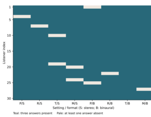
Requiring complete scores for every presentation retained twenty listeners. Each supplied six setting comparisons, yielding 120 comparisons in that restricted sample. Each of the remaining ten listeners supplied three usable comparisons. Together these observations produced 150 available comparisons from the 180 possible. Thus, a small proportion of absent answer cells reduced the number of cross-setting comparisons by one-sixth and excluded one-third of listeners from the fully complete restriction. The loss is determined by the four-presentation requirement for a comparison rather than by the overall proportion of missing cells alone.
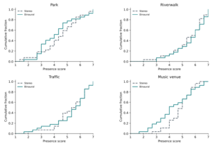
The matched empirical distributions in Figure 2 show the cumulative proportion of scores at or below each value. Their steps retain the discreteness of the three-item mean and avoid presenting smooth densities unsupported by the sample size. The two formats overlap substantially within every setting. Differences in the position and shape of the steps nevertheless show why one average shift cannot characterize every listener. These are marginal score distributions from matched people; the curves do not themselves identify which individuals changed direction.
3.2. Average paired changes and aggregate ordering
The average binaural-minus-stereo differences were negative for the ecological park and music venue, positive for the riverwalk, and numerically zero for traffic (Table 1). Every listener-bootstrap interval crossed zero. The music venue had the largest absolute point estimate, but its interval extended from a reduction of approximately one point to a small increase. The traffic estimate illustrates a different feature: equality of format means can coexist with considerable variation among paired differences. Its standard deviation of individual differences was 1.45 points despite a mean of zero.
| Setting | \(n\) | Stereo | Binaural | Difference [95% interval] |
|---|---|---|---|---|
| Ecological park | 27 | 4.46 | 4.20 | \(-0.26\;[-0.73,\,0.22]\) |
| Riverwalk | 28 | 5.46 | 5.63 | \(0.17\;[-0.32,\,0.64]\) |
| Traffic | 28 | 5.27 | 5.27 | \(0.00\;[-0.52,\,0.54]\) |
| Music venue | 27 | 4.80 | 4.33 | \(-0.47\;[-1.01,\,0.06]\) |
The descriptive ordering of average scores was riverwalk, traffic, music venue and ecological park in both formats. Restricting all setting means to the same twenty fully observed listeners preserved that order. However, the binaural averages for the last two settings differed by only 0.017 points in that common sample. The stable ordering therefore should not be mistaken for strongly separated setting effects. A small change in scores could alter the position of two nearly equal averages without indicating a substantial experiential difference.
Directional counts add information that is not contained in the means. For the park, nine listeners increased, fifteen decreased and three tied; the corresponding riverwalk counts were fifteen, ten and three. Traffic had ten increases, eleven decreases and seven ties. The music venue had ten increases, eleven decreases and six ties, although its mean difference was negative. In that case, the imbalance in the sizes of changes was more influential than the nearly balanced numbers of listeners changing in each direction. All four Holm-adjusted sign-test values were 1.00, providing no evidence of a consistent directional shift under these checks.
3.3. Cross-setting contrasts within individual listeners
Strict reversals occurred in 41 available comparisons, giving a fraction of 27.3% with a listener-bootstrap interval of 19.4–34.7%. Retained direction accounted for 56.7%, and ties for 16.0%. Excluding ties raised the reversal fraction to 32.5%, with an interval of 22.9–42.1%. The increase reflects a change in denominator rather than additional disagreements. Both summaries concern the same observed reversals, and neither can be read as a rate of technology-induced error.
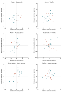
The contrast coordinates in Figure 3 display the underlying comparison geometry without replacing individual answers by setting averages. Opposite-sign quadrants contain reversals, same-sign quadrants contain retained orderings, and points on an axis contain at least one tie. Marker area increases when several listeners occupy the same coordinate. The distance of a point from both axes indicates the observed size of a reversal. This presentation separates the direction of comparison from its magnitude and makes equal contrasts visible rather than merging them with agreement.
The riverwalk–traffic comparison had ten reversals among 26 available comparisons, the largest descriptive fraction among the six pairs. Park–riverwalk and riverwalk–music each had five reversals, while park–traffic, park–music and traffic–music had six, seven and eight, respectively (Table 2). These counts identify where disagreement occurred in the present observations. They do not establish that one pair has a higher population reversal probability than another, because the comparison counts are small and share participants.
| Contrast | Available | Reversed | Retained | Tied |
|---|---|---|---|---|
| Park–riverwalk | 25 | 5 | 14 | 6 |
| Park–traffic | 25 | 6 | 18 | 1 |
| Park–music venue | 24 | 7 | 13 | 4 |
| Riverwalk–traffic | 26 | 10 | 10 | 6 |
| Riverwalk–music venue | 25 | 5 | 17 | 3 |
| Traffic–music venue | 25 | 8 | 13 | 4 |
The ordering of group means does not impose the same ordering on every person. In particular, the two settings with the highest aggregate averages also generated the largest number of reversals when compared within listeners. This is compatible with the arithmetic of aggregation: positive and negative personal contrasts can offset one another. The result therefore concerns preservation of individual comparisons, not a contradiction between two statistical summaries. Each summary answers a distinct question about the same repeated responses.
3.4. Listener weighting and the size of reversals
Twenty listeners experienced at least one reversal, and ten experienced none. Listener-specific fractions ranged from zero to two-thirds of their available comparisons. Figure 4 presents those fractions without suggesting that listeners with fewer usable comparisons have the same information as those with complete records. An observed zero means that no reversal occurred among the available comparisons; it does not demonstrate stability under repeated future listening. Similarly, a high fraction based on three comparisons should not be interpreted as a precise personal characteristic.
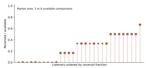
Giving every listener equal weight produced an average fraction of 25.0%, lower than the pooled comparison fraction. The fully observed restriction gave 37 reversals among 120 comparisons, or 30.8%. These results indicate that completeness and weighting affect the numerical summary. They also show that disagreement persists when incomplete listeners are excluded. Neither restriction identifies why responses were absent, and neither should be presented as automatically less biased than the other.
Twenty-four reversals retained contrasts of at least two-thirds of a point in both formats. Sixteen retained contrasts of at least one point, amounting to 10.7% of all available comparisons. The threshold profile in Figure 5 shows how the count falls as the required contrast increases. It distinguishes a reversal created by a small crossing from one involving more separated scores. This descriptive distinction strengthens the interpretation of observed disagreement while leaving its practical importance uncalibrated.
Assigning no reversals to the thirty unavailable comparisons yields 22.8% of all possible comparisons; assigning all thirty to reversal yields 39.4%. This range is a missing-information bound, not a sampling interval. It demonstrates that the observed conclusion of some disagreement cannot be removed by the missing comparisons, while the complete fraction remains unidentified without assumptions. The bound does not suggest that missing responses are especially likely to reverse, only that their outcomes are unknown.
3.5. Score construction, individual items and sequence
Median scoring produced 22 reversals, 69 retained comparisons and 59 ties. Compared with arithmetic scoring, it therefore increased the proportion of ties from 16.0 to 39.3% and lowered the inclusive reversal fraction to 14.7%. Its strict-comparison fraction was 22 divided by 91, or 24.2%. Coarser scoring changes which distinctions remain expressible. The sensitivity display in Figure 6 consequently presents denominator and scoring choices as different estimands rather than interchangeable estimates of a single fixed quantity.
Allowing two observed items retained 29 matched listeners in every setting. The resulting mean differences were \(-0.37\) points for the park, \(0.13\) for the riverwalk, \(-0.01\) for traffic and \(-0.44\) for the music venue. The broad setting pattern was similar to the complete-presentation calculation, although the park estimate became more negative. This check increases coverage by changing the scoring rule, so it cannot be interpreted as simply adding complete observations to an otherwise identical outcome.
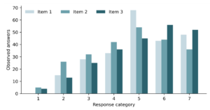
The individual-item differences in Table 3 also varied. For the music venue, the second item had a more negative difference than the other two. For traffic, the third item increased while the first two decreased. Across all presentations, the three items had 235, 239 and 231 numeric answers, respectively. Their category frequencies in Figure 7 describe the response structure underlying the composite. Those pooled counts include both formats and all settings, and therefore should not be interpreted as independent observations or as format effects.
| Setting | Item 1 | Item 2 | Item 3 |
|---|---|---|---|
| Ecological park | \(-0.28\) (29) | \(-0.37\) (30) | \(-0.41\) (27) |
| Riverwalk | \(0.24\) (29) | \(-0.03\) (29) | \(0.21\) (28) |
| Traffic | \(-0.10\) (29) | \(-0.20\) (30) | \(0.21\) (28) |
| Music venue | \(-0.29\) (28) | \(-0.80\) (30) | \(-0.36\) (28) |
The fraction of answers in categories six or seven changed by \(-8.6\), \(2.4\), \(6.0\) and \(3.7\) percentage points for park, riverwalk, traffic and music venue. The music venue therefore had a positive upper-category difference alongside a negative mean difference. This is possible because changes within and below the upper categories affect the arithmetic mean without necessarily changing threshold occupancy. Neither summary can replace the other without changing the substantive question.
After linear adjustment for relative presentation position, the setting intercepts were \(-0.29\), \(0.18\), \(-0.03\) and \(-0.46\) points in the same setting order. All four intervals crossed zero. The common position coefficient was 0.031 points per position, with an interval from \(-0.049\) to \(0.107\). The position display in Figure 8 situates that fitted association within the dispersed observations. It offers no strong evidence of a linear sequence relationship and does not establish that attention, fatigue or preceding content had no influence.
4. Discussion
4.1. What agreement must mean for a landscape comparison
The principal finding concerns the level at which agreement is evaluated. The descriptive order of the four setting averages persisted across formats, but individual setting comparisons frequently changed direction. These observations can coexist because an aggregate ordering depends on sums across listeners, whereas a personal ordering depends on the sign of one person’s contrast. Neither quantity determines the other. The result makes a specific demand on the interpretation of auditory representation: evidence of stable group summaries should not be used as evidence that the same people made the same comparisons.
This distinction has practical relevance when recordings support a conversation about places. A design team may use average responses to describe the overall impression conveyed by several materials. A facilitator may instead need to understand whether a particular participant distinguishes two alternatives consistently. Those purposes require different evidence. The first can be served by group summaries accompanied by uncertainty; the second requires linked judgments and attention to individual changes. Quantitative soundscape representation has already moved toward distributions rather than single location values [7]. The present analysis adds the cross-format linkage needed to distinguish variation among people from changes within the same people.
The observed reversals should not be interpreted as failures by participants. A questionnaire response is a situated judgment, and a changed answer may reflect an altered experience, ordinary fluctuation, attention, interpretation or the particular content made salient by the recording. Calling every reversal an error would presume a correct ordering that the experiment did not establish. There is no on-site presence ordering against which these responses can be scored. The useful result is the amount and location of disagreement under the two presentations, with its causes remaining unresolved.
The riverwalk–traffic contrast is especially instructive. It joins the two highest setting averages yet contains the largest number of reversals. This suggests that a strong-looking group hierarchy may not provide a stable personal distinction, but it does not establish that riverwalk and traffic experiences are intrinsically ambiguous. Only one recorded example represents each setting. The observed comparison could depend on the particular acoustic events captured, the duration selected or listeners’ familiarity with those events. Generalization from the recording pair to entire landscape categories would exceed the sampling design.
4.2. Presence, appropriateness and environmental benefit
A landscape representation can be convincing without being desirable. Presence concerns the experience of being situated in the represented setting; appropriateness concerns whether sounds suit a context or activity. Recent work on appropriateness and on the role of context illustrates the importance of keeping those questions distinct [29, 30]. The traffic recording’s relatively high presence mean therefore carries no implication that traffic is beneficial or suitable for a particular public space. Equally, a modest park presence score does not diminish the ecological or cultural importance of the park itself.
This separation matters because landscape architecture frequently needs to integrate evidence about comfort, restoration, accessibility and identity. Research concerning natural sounds and health addresses relationships that cannot be inferred from presence responses alone [12, 13]. The current observations contain no preference outcome, physiological result or assessment of a desired activity. Their relevance is methodological: they show how an outcome about represented experience behaves across two listening formats. Claims about environmental benefit would require direct measurements of the relevant benefit and a design capable of identifying it.
An appropriate application would state the evaluation question before choosing the recording and questionnaire. If the objective is to communicate how a place sounds, presence may be informative. If the objective is to choose a resting area, questions about calmness, disturbance or suitability are also needed. These outcomes should remain separate unless their relationship has been examined. Compatibility between quantitative and qualitative soundscape procedures likewise concerns how different forms of response contribute to evaluation rather than assuming that they express an identical judgment [31]. Short explanations from listeners could help interpret why an apparently vivid recording remains undesirable.
The three presence items also should not be regarded as interchangeable merely because they share a response range. Their differing format contrasts indicate that felt location, experienced reality and place memory do not contribute identically to every setting’s composite. The stronger negative difference for the music venue’s second item is descriptive rather than a discovery of a separate psychological mechanism. Establishing that mechanism would require a more detailed measurement study. Here, retaining item estimates prevents an arithmetic summary from concealing the aspects of presence represented in the answers.
4.3. Why spatial presentation cannot be assigned a causal advantage
Binaural playback supplies spatial cues through a representation of human hearing, but its technical description does not guarantee higher presence in every task. Spatial recording and reproduction involve choices that affect what the listener receives [4, 5]. In the current observations, the direction of the average format difference varied among settings, and the uncertainty intervals were broad. Neither the presence of spatial cues nor the numerical direction of one estimate warrants a claim of universal superiority. The defensible conclusion is confined to the observed differences and their uncertainty.
A causal account of reversals faces a more fundamental difficulty. Every setting was heard once in each format, with no same-format repetition. Consequently, the investigation cannot estimate how often listeners would reverse a comparison after two stereo presentations or two binaural presentations. An ordinary fluctuation rate could be low, high or setting-dependent; none is identified here. Comparing the cross-format fraction with an assumed value of zero would assign all temporal variability to format and would therefore misstate the design.
Randomized presentation order helps distribute sequence effects, but it does not resolve every threat to causal interpretation. The linear position adjustment addresses an average association with relative position. It does not represent a listener’s memory of a specific preceding sound, changes in engagement or differential fatigue. Nor does it demonstrate perceptual equivalence between the two recordings beyond their nominal setting labels. The fitted association is consequently a sensitivity check on a specified nuisance variable rather than a general proof that presentation history is irrelevant.
More immersive systems do not remove the need for this distinction. Work comparing virtual and real assessments, and investigations of virtual-environment ecological validity, evaluate correspondence under particular combinations of audio, visual information and interaction [16, 17]. A review of urban virtual soundscape applications similarly identifies a variety of technical configurations [32]. Those configurations cannot be ranked solely by whether they produce larger presence scores. For a design task, the relevant question is whether they preserve or improve the particular judgment needed, assessed against an appropriate external criterion.
4.4. The consequences of ties and category spacing
The change from item means to medians substantially altered the apparent rate of reversal. It also created many more ties. This is an expected consequence of reducing the number of distinct score values, but it has interpretive importance: a lower reversal fraction can arise because a scoring rule stops distinguishing settings. It should not automatically be presented as stronger agreement. Reporting retained, reversed and tied outcomes together reveals this tradeoff. A method that classifies many observations as equal may offer less comparative resolution even while generating fewer strict disagreements.
The arithmetic score uses one-third-point increments and consequently preserves more distinctions than an item median. Its greater resolution comes with an assumption about category spacing. Work on soundscape scale interpretation and ordinal modelling cautions against treating that assumption as a psychological fact [19, 20]. The sensitivity checks here do not identify a uniquely correct spacing. They show which conclusions depend on the scoring rule: disagreement remains observable, whereas its exact fraction and the balance between strict comparisons and ties change substantially.
Threshold summaries answer another question again. The upper-category fraction emphasizes whether responses cross into six or seven; a mean also reflects movement among lower categories. The positive music-venue upper-category difference alongside a negative mean difference is therefore not an inconsistency. It demonstrates that different summaries weight different parts of a distribution. Selecting a summary after inspecting which direction it produces would weaken the interpretation. Specifying the outcome before collection, and presenting alternative summaries as sensitivity checks, would provide a clearer basis for future comparisons.
The contrast threshold profile addresses a different concern from ordinal scoring. It asks whether observed reversals remain when both format-specific contrasts must exceed a stated size. Sixteen comparisons met a one-point requirement, showing that disagreement was not confined to the smallest possible crossings. However, a one-point requirement has not been linked to a planning decision, a participant’s certainty or a meaningful change in experience. Its value is descriptive transparency. Calibration against task-specific consequences would be required before it could become a decision threshold.
4.5. Sampling, missing answers and the limits of precision
Listener-level resampling preserves the repeated structure but does not create new participants or new environments. The age range is narrow, and the sample does not establish representation of people with different hearing, cultural familiarity or professional experience. A small convenience group can reveal a measurement issue without defining its prevalence in a wider public. Sample-size justification should be tied to the intended inferential target rather than to the count of repeated answers [33]. Here, the interval widths provide a more useful statement of precision than a retrospective power calculation.
The four recordings are a second limitation on generalization. There are no independently sampled parks, riverwalks, traffic corridors or music venues within each category. A participant bootstrap expresses uncertainty across listeners conditional on these stimuli; it cannot capture variation among sites. This distinction is necessary whenever repeated human observations are combined with a small fixed set of environmental materials. An expanded investigation would need replication at both levels to support claims about environmental categories or about the general behavior of a recording format.
Missingness also interacts with the comparison structure. One incomplete presentation removes the three setting-pair comparisons involving that setting for the affected listener. Complete restriction changes both the sample and its weighting. The equal-listener estimate and the pooled comparison estimate make that weighting visible, but neither reconstructs the absent judgments. The conservative missing-information bound makes fewer assumptions, at the cost of a wider range. These approaches serve complementary descriptive purposes and should not be collapsed into a claim that missingness has been corrected.
The comparison-weighted estimate is useful when the target is the available set of judgments, whereas equal-person weighting is useful when the target is the average listener’s fraction. Their numerical difference should therefore be explained through the target rather than through a search for the more favorable percentage. Both remain conditional on observed answers. Future collection could reduce this ambiguity by confirming questionnaire completion immediately after each presentation while preserving the option to decline an answer. Such a procedure would improve documentation of missingness without forcing a response or assuming why it was omitted.
The broad intervals for the mean differences require equal caution. Crossing zero is compatible with several directions and magnitudes of difference; it does not demonstrate interchangeability. An equivalence analysis would need a tolerance justified by the intended use and enough precision to evaluate that tolerance [26]. Estimation-focused practice encourages attention to plausible effect sizes rather than a binary conclusion based on statistical significance [27, 28]. In this case, the proper interpretation is uncertainty about average format differences alongside directly observed personal disagreement.
4.6. Implications for participatory listening and subsequent research
For a consultation that uses recorded environments, the immediate implication is to retain participant linkage. If responses are anonymous in a way that prevents pairing, a stable group average can conceal changes in who prefers or distinguishes an alternative. A short identifier can preserve the repeated structure without requiring personal names in the analytical record. Consistent playback arrangements and a stated response construct would then make it possible to examine the agreement relevant to the consultation. These practices follow from the measurement problem; their benefit to actual decision quality was not tested here.
The social interpretation must remain equally careful. Representations can shape participation through their selection and presentation [2], while landscape sound interventions involve choices about where and how acoustic experience is addressed [34]. The present findings provide no direct observation of persuasion, exclusion or workshop deliberation. They do identify a point at which a facilitator might pause before describing a group average as consensus. A distribution of linked judgments can reveal disagreement that deserves discussion without presuming which judgment should prevail.
A subsequent listening investigation could cross multiple independent recordings with repeated presentations in each format. Same-format repetitions would estimate ordinary response fluctuation; cross-format repetitions would permit comparison with that fluctuation. Sampling several locations within each environmental category would distinguish variation among places from variation among recordings. On-site judgments would supply an external point of comparison for the intended construct, while separate questions about preference and appropriateness would prevent presence from carrying evaluative meanings it does not possess.
Audio and visual components would also need to be considered together when the intended application includes images or movement. Research on water features and traffic demonstrates that audio-visual assessment can involve interactions absent from sound-only listening [35]. The ecological-validity literature similarly supports testing the actual presentation conditions rather than extrapolating from a different apparatus [18]. The current eyes-closed observations isolate neither every auditory mechanism nor the full experience of landscape, but they provide a precise account of what happened within the available listening task.
4.7. Transfer to visual and culturally diverse assessment
The present interpretation also depends on the restriction to eyes-closed listening. In a consultation, recordings may accompany a photograph, model or moving image. Visual information can identify a location, supply expectations about sound sources and redirect attention toward particular events. Comparisons of visual presentation methods in virtual landscape and soundscape evaluation provide a reason to test these combinations directly [36]. A result from an auditory-only task cannot determine whether adding images would stabilize comparisons, amplify differences or change the outcome being judged. That question requires linked observations under the intended presentation conditions.
Restorative interpretation requires the same restraint. Investigations of birdsong and perceived restoration address a more specific evaluative outcome than feeling present in a recording [37]. Their relevance here is to the selection of questions, not to an inferred health effect in the thirty listeners. If a design process aims to compare opportunities for recovery, its listening protocol should directly assess that aim and distinguish it from spatial vividness. Collecting both outcomes would permit their association to be examined rather than assuming that one stands for the other.
Cultural transfer introduces another source of uncertainty. A seven-category response form can appear numerically identical across languages while its terms carry different associations. Research translating soundscape attributes illustrates why linguistic validation is part of measurement design [38, 39].
These considerations define a practical sequence for evaluating an auditory comparison. The intended decision determines the response construct; the presentation conditions determine which aspects of place are available; and linked answers determine whether personal contrasts persist. Evidence from one stage cannot silently substitute for evidence from another. A recording can be technically consistent yet unsuitable for an evaluative question, and a questionnaire can be clear yet insufficiently sensitive to distinguish alternatives. The contribution of the current analysis is to expose one measurable relationship within that sequence, rather than to certify an entire consultation procedure.
5. Conclusion
The four recorded settings retained the same descriptive ordering of average presence scores across stereo and binaural playback, while individual comparisons were less stable. More than one-quarter of available within-listener setting comparisons reversed direction, and sixteen reversals retained contrasts of at least one point in both formats. The occurrence of disagreement persisted after restriction to fully observed listeners, although its numerical fraction depended on listener weighting, denominator choice and scoring. Median scoring reduced reversals partly by producing more ties.
These findings answer the central question by showing that aggregate ordering alone is insufficient evidence of preserved individual comparisons. They do not establish that recording format caused the reversals, that one format was superior, or that the settings differed in preference or restorative benefit. The absence of same-format repetitions and on-site assessments prevents those interpretations. For landscape architecture, the appropriate response is to evaluate recorded representations against the comparison required by their use, retain linked observations, and distinguish presence from environmental value. A technically convincing presentation should be judged by the fidelity of the relevant decision evidence rather than by its average presence score alone.
Declarations
Author Contributions
All authors contributed equally to this study. All authors read and approved the final version of the manuscript for publication.
Conflict of Interest
The authors declare no conflicts of interest.
Funding Information
This research received no external funding.
Data Availability
The data used in this study are available from the corresponding author upon reasonable request.