
1. Introduction
The depth specified for a sand cap has consequences that extend well beyond the moment when material is spread. It determines an imported volume, affects the conditions encountered by emerging vegetation, and can alter the work required to keep a new meadow within its intended composition. These consequences are often assessed in different parts of a landscape commission. A construction estimate addresses supply and placement, a planting specification addresses establishment, and a maintenance contract addresses subsequent care. Bringing those commitments into the same calculation is necessary when a design is justified partly by the expectation of reduced upkeep. A meadow can demand less routine attention than an intensively maintained landscape while still requiring considerable intervention during its first growing season.
The need for careful establishment is strengthened by the broader decline of biodiversity and by recognition that restoration must include open, herbaceous ecosystems as well as wooded vegetation [1, 2]. Within cities, relatively small areas can support native plants and associated organisms when vegetation structure and species selection are appropriate. Evidence from changes to urban understoreys and small greening interventions demonstrates the value of attending to these attributes [3, 4]. Such findings justify investment in planted vegetation, but they do not make all methods of producing it interchangeable. A material-intensive route to a flower-rich appearance may carry a different maintenance demand and a different off-site burden from a less intensive route producing comparable establishment.
Urban meadow research has documented benefits across several biological and social dimensions. Comparisons with short-mown grassland show responses in multiple groups of organisms, while replacing roadside shrub beds with wildflower planting can combine increased insect abundance with lower maintenance expenditure [5, 6]. Meadow creation within a university landscape has also connected biodiversity gains with management and cultural outcomes [7]. These studies make the practical case for considering meadow vegetation in a wider range of public settings. However, the relevant comparison during detailed design is often between alternative establishment specifications for the same planting, rather than between a meadow and a completely different vegetation type.
That distinction matters because low maintenance is not an intrinsic property conferred by a planting name. Evidence on lawn management links intervention intensity to ecological and economic outcomes, and reduced mowing can allow plant richness to increase [8, 9]. Research on arthropods likewise indicates benefits from less frequent cutting, while the timing and type of mowing affect the organisms present after an operation [10, 11]. These relationships concern established vegetation and particular management practices. They cannot directly quantify the hand-weeding that follows sowing on a disturbed urban surface. Establishment and continuing management need separate accounts, with clearly specified tasks and time horizons.
A sand cap offers one means of modifying the conditions under which seedlings and weeds compete. Burial of an existing weed seed bank and the creation of a nutrient-poor surface can change recruitment, but success remains contingent on species tolerances, moisture, and subsequent plant interactions. Ecological planting design therefore depends on the requirements of individual species as well as general community principles [12]. Evidence on urban grassland restoration also identifies soil conditions, propagule availability and management as interacting determinants of establishment [13, 14]. A deeper layer may suppress unwanted emergence more effectively, yet the extra material must be assessed against the benefit already achieved by a shallower layer.
This marginal comparison is easily obscured when the most intensive treatment is judged only against uncapped soil. The full reduction in weeding can make a deep cap appear compelling even when much of that reduction is already available from a thin application. For a contractor or public client, the relevant question after accepting the thin cap is how much additional work the next volume avoids. An answer in hours saved per cubic metre can be combined with local installed prices without asserting that historical labour measurements and current quotations share the same monetary context. It can also reveal cases where the financial return on additional material is small even though the total treatment effect is large.
The environmental consequences of sand consumption provide a further reason to distinguish total benefit from marginal return. Sand moves through supply systems whose effects are not visible within the receiving planting. Research on material movement and constructed urban soils shows why an ecological appearance cannot establish the sustainability of the materials used to create it [15, 16]. Studies of the global sand system, riverine extraction and resource governance identify consequences extending beyond purchase price [17–20]. A cap-volume calculation is not a substitute for environmental assessment, but it makes a consequential physical input explicit before that assessment begins. Avoided weeding and imported sand should remain visible in their respective units.
Jute complicates this comparison because it introduces a second material and may influence more than one component of establishment. A mesh treatment can be attractive when it is expected to retain seed or modify the germination surface. Those expectations do not establish that its labour saving remains useful at every sand depth. Nor do they establish that the plant community responds uniformly. A treatment might reduce weeding while also reducing the number of forbs successfully retained in the sampled vegetation. Treating richness as a separate endpoint prevents a small financial advantage from concealing that ecological consequence.
Plant richness nevertheless requires a precise interpretation. Species counts do not measure nectar production, flower continuity or animal use. Urban pollinator research demonstrates that resources and interactions depend on the plants and habitats available, while nectar production varies among flowering taxa and landscape settings [21–23]. Similarly, responses to native vegetation depend on plant identity and structure rather than species totals alone [24]. In a construction comparison, pooled forb richness can act as a check on taxonomic establishment, but it cannot certify the full ecological performance of a meadow. It is especially important to distinguish a count from small quadrats from an inventory of the complete planted area.
Public expectations introduce another independent consideration. Meadow appearance can affect perceptions of site quality, and implementation decisions involve staffing, location, public response and financial constraints [25, 26]. The colour and diversity perceived by visitors are not necessarily the diversity counted by a vegetation survey [27]. Consequently, assigning a single monetary value to each additional species would imply a level of agreement among ecological, aesthetic and operational aims that these measurements cannot support. A clearer decision is to define the planting requirements first and compare construction costs among the alternatives that remain acceptable.
The distinction between construction and care also affects what constitutes success in a field comparison. A visually complete surface can conceal substantial selective labour, while a diverse planting can remain operationally difficult if unwanted vegetation must be removed during a narrow window. Conversely, reducing recorded work is not sufficient if the treatment moves the vegetation away from the intended forb component. These competing outcomes make a single ranking difficult to defend. A useful analysis must preserve the separate evidence for construction demand, actual work and plant establishment, and then state how a financial comparison combines only the relevant quantities. This is particularly valuable for native meadow projects, where ecological ambition can be high but the available establishment budget is fixed. The specification should make the exchange visible before construction commits the client to either material delivery or future selective care.
The present analysis asks when additional sand is compensated by avoided establishment-weeding expenditure and whether adding jute changes that calculation at an ecological cost. It uses assigned construction treatments, actual weeding minutes and twelve-month species counts from a randomized Melbourne experiment. The analytical contribution is a set of marginal material-to-labour exchange rates and a comparison of competing treatment costs, with uncertainty retained at the plot level. It does not claim that sand-induced weed suppression or jute-related community changes are new discoveries. Its purpose is to translate the measured treatment responses into quantities that can be interrogated during specification, procurement and establishment budgeting.
The comparison is deliberately confined to the three tested depths. No performance is assigned to intermediate layers, and no future maintenance saving is inferred by repeating the first-year observations. Arithmetic labour totals are used because hours accumulate across plots and visits. Forb richness remains outside the financial equation. The resulting account addresses a practical question within landscape architecture: how should a client distinguish easier maintenance from efficient use of construction material when both are legitimate objectives? The answer must state the relative prices at which choices change, the ecological consequences of mesh, and the limits imposed by an irrigated experiment at one site.
2. Materials and Methods
2.1. Experimental setting and treatments
A field experiment in Royal Park, Melbourne, Australia, examined urban meadow establishment under different combinations of sand depth and jute application [28]. The present study analyses weeding demand and forb richness during the 2020–2021 establishment period. The site was located at approximately 37\(^\circ\)47\(‘\)34\(”\) S and 144\(^\circ\)57\(‘\)21\(”\) E. Fifty-four plots, each measuring 24 m\(^2\), were randomly assigned to six treatment combinations comprising three sand depths (0, 10 and 80 mm), each with or without jute. Every combination contained nine plot replicates.
A native mixture of 22 forb and five grass species was sown in April 2020 at 2.73 g m\(^{-2}\). Jute had a nominal areal mass of 500 g m\(^{-2}\), and irrigation supplied approximately 2.85 mm daily through May 2021. Hand-weeding time was measured during six visits between July 2020 and May 2021, excluding the removal of elm suckers and eucalypt seedlings. Vegetation counts were recorded at six and twelve months in four fixed 0.25 m\(^2\) quadrats per plot. The ecological endpoint examined here uses the twelve-month survey.
Labour requirements and plant establishment are interpreted in relation to the irrigation regime, seed mixture and specified weeding task. Irrigation could influence both sown and unwanted vegetation, while the species mixture defined the potential contribution of sown taxa to richness. Transfer to rain-fed meadows, alternative mixtures or established grasslands managed through periodic mowing therefore requires further evidence. Restoration standards and seed-supply research similarly emphasize ecological targets, planting material and treatment conditions when assessing the applicability of management prescriptions [29–31].
2.2. Observation checks and sampling support
The analysis includes 324 plot-visit labour measurements and 216 quadrat observations, with six distinct visits and four distinct quadrats represented for every plot. Before observations were linked, the alternative soil label SO was standardized to S0 without changing measurement values. Treatment groups remained balanced. Labour measurements and forb counts were complete and nonnegative, and species-count fields contained integer values.
Plots were the units of treatment assignment and replication. Repeated visits describe maintenance within the same plot, while quadrats characterize vegetation within it; neither provides additional independently assigned replicates. Uncertainty estimation therefore retained the distinction between repeated measurements and experimental units [32]. Labour was summed and species occurrences were pooled within plots before treatment means were calculated and bootstrap samples drawn. Plots with unusually high weeding requirements were retained.
Quadrat-derived twelve-month forb cover differed from the corresponding plot-level summaries in three plots by \(-2.50\), \(-1.50\) and \(-0.25\) percentage points. Cover was therefore excluded from the principal labour and ecological comparisons. Richness was calculated independently from species counts and was unaffected by these discrepancies. Slug abundance, which included one missing observation, was outside the selected endpoints.
Together, the four quadrats sampled 1 m\(^2\) within each planted plot. Pooling their species occurrences produced one richness value per experimental unit and represented a larger sampled area than an individual quadrat. Mean quadrat richness was also calculated to assess whether the direction of the jute contrast depended on pooling. Both measures describe richness within the sampled vegetation and remain sensitive to sampling effort; neither constitutes a complete inventory of the plot.
2.3. Labour and construction quantities
For plot \(i\), cumulative labour was calculated by adding the six observed visit times before converting minutes to hours and standardising the area. With \(t_{iv}\) denoting minutes at visit \(v\), the accounting quantity was
Its unit is hours per 100 m\(^2\). This conversion facilitates comparison with material quantities; it does not demonstrate identical productivity on a larger construction contract. Travel, mobilisation, task supervision and other fixed costs could prevent direct scaling from a small plot to a municipal planting. Treatment means are untransformed arithmetic means, appropriate to an additive labour budget, rather than means of logarithms or predictions from a transformed response model.
A depth \(d_k\), measured in millimetres, requires a nominal sand-cap volume \(V_k=0.1d_k\) cubic metres per 100 m\(^2\). The three assigned depths therefore correspond to 0, 1 and 8 m\(^3\) on this accounting basis. Where jute was present, coverage was 100 m\(^2\) and nominal mass was 50 kg. These are specified quantities, not measured delivery totals. Settlement, compaction, overlap, edge detailing and wastage were unavailable. Sand used in common as a seed carrier was excluded from the differential cap comparison because the calculation concerns the additional surface layer.
The timing of work was described using mean hours at each visit and the proportion of treatment labour accumulated during the first two visits. That proportion was computed from pooled treatment minutes, so it describes the share of all recorded work rather than the average of nine plot-specific percentages. Empirical exceedance curves were also calculated for unmeshed plots. At a given number of hours, the curve gives the fraction of observed plots requiring more time. These curves describe the sample and were not fitted as forecasts of future workload.
2.4. Forb establishment and marginal comparisons
Let \(n_{iqs}\) be the twelve-month count of forb species \(s\) in quadrat \(q\) of plot \(i\). Pooled richness was
A species was counted once if present in any sampled quadrat. The endpoint gives equal presence weight to sparse and abundant taxa, excludes the five sown grasses, and does not weight conservation status, flowering duration or functional traits. Its role is to retain one clearly defined component of establishment alongside labour and material demand. No currency conversion was applied to richness, and no numerical threshold of acceptable diversity was imposed.
Successive sand increments were compared within each jute condition. The first increment added one cubic metre per 100 m\(^2\); the second added seven. Labour savings were calculated as the shallower-treatment mean minus the deeper-treatment mean. The mesh comparison was calculated within each sand depth, using the unmeshed mean minus the meshed mean for labour and the meshed mean minus the unmeshed mean for richness. Positive labour differences thus indicate avoided work, whereas negative richness differences indicate fewer established forb species under mesh. These sign conventions keep the resource saving and ecological change distinct.
2.5. Installed prices and competing treatment costs
The financial comparison uses the fully burdened hourly labour price \(w\), the installed sand price \(c_s\) per cubic metre, and the installed jute price \(c_j\) per square metre. Defining \(u=c_s/w\) and \(v=c_j/w\) gives price ratios in h m\(^{-3}\) and h m\(^{-2}\). For treatment \(k\), the attributable cost divided by \(w\) is
where \(A_k\) is either zero or 100 m\(^2\). The expression includes recorded weeding and the two differentiated construction inputs. It excludes unmeasured treatment-specific work and all common expenditure. Installed material prices must cover acquisition, delivery and placement; adding those activities again as separate labour would count them twice.
For alternatives \(a\) and \(b\) sharing the same mesh condition, with \(V_b>V_a\), the break-even sand ratio is
The deeper cap has lower accounted cost when \(u<u^*\). At a fixed depth, the mesh ratio is \(v^*=(\overline H_N-\overline H_J)/100\). Pairwise equality does not guarantee that either treatment is cheapest among all six options. Accordingly, the analysis also takes the minimum of the six cost expressions at each pair of nonnegative price ratios. The graphical price slice fixes \(v\) at 0.05 h m\(^{-2}\) and varies \(u\); this is an explicit arithmetic illustration, not an observed quotation.
A further distinction concerns construction feasibility and economic preference. The cost equation assumes that all compared treatments can be installed under the same project conditions. If a treatment cannot meet a drainage, access or procurement requirement, it should be excluded before taking the minimum. Otherwise a mathematically inexpensive treatment could enter a ranking despite being unavailable to the commission. The equation also assumes positive labour prices and nonnegative installed material prices. It does not include subsidies, resale values or savings from combining deliveries with another project. Such adjustments can be added when documented, but they should retain their own units and avoid changing the observed weeding totals. The comparison is thus open to local financial information while keeping the empirical labour component fixed.
No discount rate was applied because a dated sequence of actual payments and comparable local prices was unavailable. The calculation is an establishment-period account in common price units. It cannot be interpreted as a discounted life-cycle appraisal. Treatment-specific differences in irrigation, access, removal of waste or subsequent renewal would require additional terms. Keeping these omissions visible is preferable to assigning unsupported prices to activities that were not measured.
2.6. Uncertainty and sensitivity
Uncertainty was evaluated using 50,000 nonparametric bootstrap resamples, drawing nine whole plots with replacement independently within each treatment. Labour and richness from a selected plot remained together. Percentile intervals were formed from the 2.5th and 97.5th percentiles of treatment means and their contrasts. The main summaries used random seed 20261031. The continuous selection-stability illustration used the same seed with treatment draws ordered as the six curves appear. It is a separate Monte Carlo evaluation of the same resampling procedure.
Percentile intervals are transparent but can have imperfect coverage with small, skewed samples; a large number of resamples does not create additional field replication [33, 34]. The intervals are exploratory and are not adjusted for all simultaneous comparisons. They indicate precision conditional on these observations, rather than certifying a binary distinction between meaningful and meaningless effects [35]. In particular, overlap or proximity of richness means cannot establish equivalence without an ecological margin and a corresponding test [36].
Each plot was also deleted once to recalculate the unmeshed sand thresholds. This check identifies dependence on influential observations without automatically excluding them. Median-based thresholds were calculated separately to show how the answer changes when the planning target becomes a typical plot rather than expected aggregate labour. Finally, bootstrap cost rankings were evaluated at selected fixed price ratios and along the graphical price slice. Selection frequencies quantify sensitivity to resampling the observed plots; they are not probabilities that a treatment will succeed at another location.
3. Results
3.1. The amount and timing of establishment work
The six visits accumulated 6897.72 minutes of hand-weeding across the 54 plots, equivalent to 114.96 hours on the actual experimental area. Standardisation to 100 m\(^2\) gave treatment means ranging from 4.28 to 19.44 hours over the establishment period. Without jute, mean labour fell by 49.8% between uncapped soil and the 10 mm cap, and by 76.1% between uncapped soil and the 80 mm cap. With mesh, the corresponding reductions were 28.5% and 51.4%. The mesh treatments therefore started from a lower uncapped labour demand and offered a smaller absolute saving from additional sand.
The uncertainty in uncapped, unmeshed labour was substantially greater than that of the deepest cap, as shown in Table 1. Its standard deviation was 15.33 hours, compared with 4.34 at 10 mm and 1.29 at 80 mm. The width of the interval is thus a substantive feature of the observed work distribution, rather than simply a consequence of unequal sample size. All treatments had the same number of independently assigned plots. Mean labour under mesh also became less variable with increasing depth, with standard deviations of 4.01, 2.03 and 1.22 hours, respectively.
The visit sequence shows where those totals accumulated (Figure 1). Across treatments, the second visit required 2336 minutes, the largest pooled total, followed by 1331 minutes at the first and 1240 at the third. The last visit required 494.46 minutes. Differences between treatment totals consequently cannot be understood solely as a constant saving repeated at each visit. Construction altered the early concentration of work as well as its cumulative amount.
| Depth; mesh | Sand m\(^3\) | Jute kg | Weeding hours per 100 m\(^2\) | Pooled forb species per plot sample |
|---|---|---|---|---|
| 0 mm; absent | 0 | 0 | 19.44 (11.71–29.98) | 8.78 (7.33–10.22) |
| 10 mm; absent | 1 | 0 | 9.76 (7.46–12.68) | 8.44 (7.11–9.78) |
| 80 mm; absent | 8 | 0 | 4.65 (3.86–5.43) | 8.56 (7.33–9.78) |
| 0 mm; present | 0 | 50 | 8.80 (6.61–11.55) | 6.44 (5.44–7.44) |
| 10 mm; present | 1 | 50 | 6.29 (5.17–7.65) | 7.78 (6.78–8.78) |
| 80 mm; present | 8 | 50 | 4.28 (3.57–5.06) | 6.44 (5.89–7.00) |
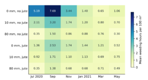
The first two visits accounted for 66.3% of all labour on uncapped soil without jute, compared with 54.4% at 10 mm and 39.8% at 80 mm. Under mesh, their shares were 44.2%, 41.8% and 40.4%, respectively. These percentages describe the timing of treatment totals and do not imply that every plot followed the same trajectory. They nevertheless show that the high uncapped mean was associated with a pronounced early obligation. The deepest cap reduced that concentration under the recorded visit schedule.
3.2. Differences between expected and typical labour
The empirical exceedance curves reveal a long upper tail in uncapped, unmeshed demand (Figure 2). Its maximum was 56.59 hours per 100 m\(^2\), while its median was 13.62 hours. The corresponding maxima were 19.40 and 6.53 hours for the two sand depths. Mean and median were much closer under the 80 mm cap, with a median of 4.80 hours against a mean of 4.65. These observations distinguish the expectation used for aggregate budgeting from the time required by a typical plot.
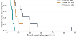
The curves do not justify a guaranteed upper limit on future work. Nine plots can reveal observed heterogeneity but cannot reliably estimate the extreme tail of a municipal planting programme. Their value is diagnostic: the uncapped treatment exposed the experiment to a much wider range of labour requirements. A financial comparison based on medians would underweight that observed tail, whereas a comparison based on means retains it. Both summaries are useful when their different planning purposes are stated.
3.3. Successive sand increments
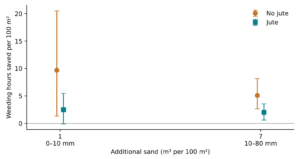
The first unmeshed sand increment saved 9.68 hours per 100 m\(^2\), with a percentile interval of 1.33–20.51. The second saved 5.10 hours, with an interval of 2.66–8.15, despite requiring seven times as much additional material. Their mean labour returns per cubic metre were therefore 9.683 and 0.729 hours. The first increment provided approximately 13.3 times the labour saving per cubic metre of the second. This ratio describes the two assigned increments and should not be interpreted as a continuous depth-response function.
The same ordering occurred with jute, although the savings were smaller (Figure 3). Moving from uncapped soil to 10 mm saved 2.51 hours, with an interval from \(-0.09\) to 5.48. Moving from 10 to 80 mm saved 2.01 hours, with an interval of 0.62–3.56. Their respective break-even ratios were 2.505 and 0.288 h m\(^{-3}\). The interval for the thin-cap mesh increment included zero, showing that its positive mean saving was less precisely resolved than the corresponding unmeshed comparison.
The material difference also has a useful proportional interpretation. A thin cap used one eighth of the sand required by the deepest cap, while delivering approximately two thirds of the total mean labour reduction available between uncapped soil and the deepest unmeshed treatment. The remaining third of that reduction required the remaining seven eighths of the cap volume. These proportions explain why a deep cap can be attractive where maintenance hours are especially scarce, yet difficult to justify where imported material is costly or constrained. They do not establish a universal efficiency score: the proportions depend on the uncapped comparator and the selected labour endpoint. Their purpose is to expose the physical asymmetry between the two increments already quantified in hours and cubic metres.
A comparison directly from 0 to 80 mm gave an unmeshed break-even ratio of 1.848 h m\(^{-3}\). That quantity exceeds the marginal threshold for moving from 10 to 80 mm because it includes the particularly productive first cubic metre. It would therefore be misleading to use the full-depth threshold to justify the final seven cubic metres after the thin cap had already been accepted. The successive increments answer different procurement questions, even though they share the same uncapped and deep-cap observations.
3.4. Jute savings and forb retention
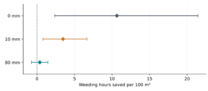
Adding mesh reduced mean labour by 10.64 hours on uncapped soil and 3.46 hours at 10 mm, with intervals of 2.36–21.44 and 0.79–6.65, respectively. At 80 mm, the estimated reduction was only 0.37 hours, with an interval from \(-0.74\) to 1.45 (Figure 4). The associated mean break-even mesh ratios were 0.1064, 0.0346 and 0.0037 h m\(^{-2}\). The financial room available for purchasing and installing jute thus narrowed sharply with sand depth.
Pooled forb richness under mesh was lower by 2.33 species on uncapped soil and by 2.11 species at 80 mm, with intervals of \(-4.11\) to \(-0.67\) and \(-3.44\) to \(-0.78\). At 10 mm, the difference was \(-0.67\) species, with an interval from \(-2.33\) to 1.00 (Figure 5). The deepest mesh treatment therefore combined an unresolved small labour advantage with a more clearly negative richness contrast. Mean quadrat richness gave the same ecological direction at that depth, falling from 4.36 to 2.81 species when mesh was present.
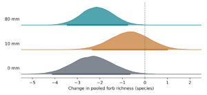
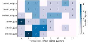
The richness distributions show that similar means did not imply identical observations (Figure 6). Unmeshed samples ranged from 6 to 12 species on soil and at 10 mm, and from 5 to 12 species at 80 mm. Meshed samples ranged from 5 to 9, 5 to 11 and 5 to 8 species, respectively. The mean differences between unmeshed depths were small relative to their uncertainty. Those results do not establish that sand depth had no ecological effect, and they do not demonstrate equivalence of the plant communities.
3.5. Price-dependent ranking and its stability
Fixing the mesh ratio at 0.05 h m\(^{-2}\) adds five labour-equivalent hours to every meshed treatment. The resulting price slice changes the least-cost choice from the deep unmeshed cap to the thin unmeshed cap and eventually to uncapped soil with jute as sand becomes dearer (Figure 7). The mean crossings occur at the marginal thresholds already calculated. The uncapped mesh treatment enters the minimum when the sand ratio exceeds approximately 4.044 h m\(^{-3}\). The displayed vertical separation is an accounted cost difference, not an ecological ranking.
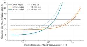
The crossings can be checked directly from the treatment means. At a sand ratio of 0.5 and the fixed mesh ratio, the deep unmeshed cap has an accounted cost of 8.65 labour-equivalent hours, compared with 10.26 for the thin unmeshed cap. Raising the sand ratio to one changes those values to 12.65 and 10.76, reversing their ordering. At a ratio of five, uncapped soil with mesh costs 13.80 labour-equivalent hours, below the thin unmeshed value of 14.76. These calculations illustrate why treating each additional material independently is insufficient when alternatives compete simultaneously. An option can be preferable to another within a pair and still be displaced by a third choice. The same equations allow a client to repeat the comparison using a quotation, while preserving the measured labour totals and the separate richness results. None of these arithmetic examples assigns a market price or predicts vegetation beyond the observed establishment conditions.
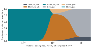
Resampling smooths those sharp mean-based transitions because each draw supplies different treatment means (Figure 8). At \(u=1\) and \(v=0.05\), the thin unmeshed cap ranked first in 81.4% of the principal bootstrap draws. At lower mesh prices, the ordering could change: at \(u=0.5\) and \(v=0.01\), the thin meshed cap ranked first in 80.7%. Near the expensive-sand boundary, uncertainty remained substantial. At \(u=10\) and \(v=0.16\), uncapped unmeshed soil ranked first in 56.0% of draws and the thin unmeshed cap in 43.9%.
Deleting one plot at a time moved the unmeshed deep-cap threshold between 0.556 and 0.789 h m\(^{-3}\). The thin-cap threshold varied more widely, from 5.040 to 11.296. Median-based thresholds were 5.974 and 0.407 for the successive increments. The exact financial boundary therefore depended on the labour summary and influential observations, while the decline in labour return per additional cubic metre remained. The smaller deletion range for the second increment does not remove its sampling uncertainty, but it shows that its mean estimate was less dependent on one extreme plot.
4. Discussion
4.1. A construction increment must earn its own saving
The central finding is a marked difference between minimising weeding hours and obtaining the greatest labour relief from a unit of imported sand. The deepest unmeshed cap performed best on the first objective, while the initial thin layer performed best on the second. These are distinct design priorities, and neither can be inferred from the other. The practical advantage of the marginal calculation is that it identifies the extra commitment under consideration. Once a thin layer is accepted, the remaining decision concerns seven further cubic metres and the work they avoid, rather than the entire contrast with uncapped soil.
This reading changes how a favourable treatment result should enter a specification. A statement that deeper sand reduced weeds or maintenance establishes a direction of response. It does not establish that every additional cubic metre is financially justified. The unmeshed threshold expresses the latter condition in a transferable unit: the installed price of an extra cubic metre must be below the price of approximately three quarters of an hour of weeding labour for the deep cap to outperform the thin one in the mean account. The large interval around that boundary requires the comparison to be treated as conditional rather than exact.
A quotation can be applied without rewriting the ecological analysis. Dividing the complete installed sand price by the fully burdened labour rate produces the required ratio. The ratio must represent the relevant work, including transport, placement and any associated handling already included in the quotation. A low supply-only price would give an incomplete comparison if spreading were then omitted. Conversely, adding placement labour separately after using an installed price would inflate construction expenditure. The value of a transparent equation is that these accounting choices become inspectable before the design team selects a treatment.
The treatment comparison remains discrete. Observing diminishing labour returns between the assigned depths does not identify the performance of a layer between them. Biological responses may be nonlinear because germinating weeds encounter burial depths, moisture gradients and competition that do not change proportionally with cap thickness. An intermediate layer could be useful, but it requires observation. The present calculation can direct attention towards that test without assigning unsupported outcomes to unmeasured depths. Landscape design benefits from this restraint because an apparently precise optimum would otherwise disguise a speculative biological response.
4.2. Budgeting for the establishment peak
The labour distributions add a second operational issue to the material comparison. A treatment with a high upper tail may create staffing difficulties beyond those conveyed by its mean. In the uncapped treatment, an unusually demanding plot raised the expected budget appreciably above the median. That observation should neither be erased as inconvenient nor promoted into a universal forecast. It shows that large work demands occurred within this trial and that the mean-based thin-cap threshold depends partly on avoiding them. The deletion check quantifies that dependence while preserving the observations in the principal calculation.
Public landscape programmes can have different reasons to prefer a mean, a median or a reserve allowance. The mean is appropriate when work can be pooled across many comparable areas and the concern is their total expected demand. The median describes a typical area but will understate an additive budget when occasional difficult areas consume much more time. A reserve allowance addresses the consequence of overruns but requires a credible estimate of the relevant tail and an explicit service objective. The present sample supports the first two descriptions; it does not establish a reliable municipal reserve rule.
Timing also matters. A high concentration of weeding during the first two visits could coincide with other seasonal responsibilities, making staff availability more restrictive than the annual wage bill. The thin cap reduced the pooled early share, and the deep cap reduced it further. Nevertheless, the value of releasing staff during those visits was not measured. Crew scheduling, access to skilled weed identification, and the possibility of delaying tasks could all affect the benefit. These questions connect directly to the staffing and economic concerns already identified in local-authority decisions about meadow adoption [26].
The term low maintenance should therefore be attached to a task and a period. Evidence that reduced mowing can benefit biodiversity and expenditure does not mean that newly sown native vegetation should receive less selective care at every stage. A recent review of maintenance and urban biodiversity shows that associations depend on the activity, organism group and context [37]. Here, the measured activity was hand-weeding during establishment. Keeping that description precise prevents the sand treatment from being credited with savings in mowing, irrigation or renewal that were never observed.
4.3. Why the mesh decision cannot be settled by cost alone
The deep-cap mesh comparison is especially instructive because it separates a numerical minimum from a convincing planting choice. When only mean weeding is considered, jute has a slight advantage at that depth. Once purchase and installation are charged, the permissible mesh price is very small. At the same time, the richness comparison indicates fewer established forbs. A design team seeking a diverse forb component would therefore have a clear reason to scrutinise this option even before adding environmental or aesthetic considerations. The result does not condemn jute in every landscape application; it identifies a weak establishment trade-off under the conditions tested.
The thin-cap comparison is less decisive ecologically. Its richness interval spans both a loss and a modest gain, so the available precision cannot resolve the contrast in the same way. Treating that interval as proof of harmlessness would be incorrect. An equivalence claim requires a defensible margin specifying how much change the planting objective can tolerate, together with sufficient precision to assess it. Such a margin was not established before this analysis. The ecological interpretation must therefore distinguish an unresolved contrast from a demonstrated absence of consequential change.
Richness also leaves species identity and abundance open. Losing one common, widely distributed forb and losing a locally scarce taxon have the same effect on the arithmetic count, but potentially different conservation consequences. Two treatments can have identical richness while supporting different species or flowering schedules. Evidence from indigenous urban plantings and pollinator interactions illustrates why plant choice can matter beyond the number of taxa [21, 24]. Future specification trials should record species-specific persistence, reproductive performance and flower availability alongside labour. Those observations would permit more direct evaluation of the intended plant community without requiring a composite score.
Visual quality needs its own evidence as well. A richness survey cannot establish what visitors notice or prefer. Perceptions can depend on colour, flowering density, season and the legibility of care, while the counted diversity may be only partly visible [25, 27]. The measured forb losses should therefore be understood as taxonomic establishment effects, not automatically as equivalent losses of public approval or amenity. This distinction protects both ecological interpretation and design judgement from claims that the available measurements cannot support.
4.4. Material efficiency and environmental responsibility
The low marginal return from the final seven cubic metres provides a useful reason to examine procurement carefully. It does not establish that the thin cap has the smallest environmental burden. Volume alone cannot identify extraction damage, processing energy, travel distance or the suitability of alternative materials. The broader literature on sand resources and the strategic recommendations for reducing unsustainable consumption make these questions relevant to small projects as well as major construction [17, 38]. A treatment can be economical within the receiving site while shifting consequences to a quarry, river or transport corridor.
Material efficiency is consequently a narrower claim than sustainability. In this experiment, the thin cap avoided more recorded labour per cubic metre than the deep cap. To compare environmental performance, the material would need a documented origin, delivery distance, processing history and any treatment-specific disposal or renewal requirements. Jute likewise requires information on cultivation, manufacture, installation and its subsequent condition. No carbon conversion was applied because reliable factors tied to the actual materials were unavailable. Assigning a generic emissions value would add apparent precision without resolving the most consequential local differences.
Urban meadow climate effects should also be assessed directly rather than inferred from appearance or reduced work. Comparisons of lawns and meadows show that greenhouse-gas exchange and drought responses depend on vegetation, soils and management [39]. Neither fewer weeding hours nor more forb species determines the complete carbon balance. The present account identifies physical material quantities and one labour obligation; these can contribute to a later environmental assessment, but they cannot replace measured or appropriately modelled exchanges. This separation is particularly important where a meadow is promoted simultaneously for biodiversity and climate objectives.
4.5. From one planting to a municipal decision
Transfer requires more than substituting a local wage. Weed pressure, seed-bank composition, climate, irrigation, sand properties, plant mixture and the methods used by workers can all alter labour savings. The comparison is strongest for the randomized plots under their common establishment conditions. It becomes less certain as an application departs from those conditions. Urban biodiversity planning must also attend to habitat area, spatial arrangement and the wider management of green space [40, 41]. A construction treatment that performs well in a plot does not establish the ecological contribution of a meadow network across a city.
The area conversion deserves particular care during transfer. A hundred square metres is an accounting basis, not the size of an independently replicated treatment area. Larger contracts may permit efficient machinery, while constrained public sites may involve additional mobilisation or restricted access. Small plots can also have edge conditions unlike those of larger meadows. The observed hours should therefore serve as a conditional productivity input, checked against local work methods, rather than an unquestioned rate to multiply across hectares. Nominal sand volume can be scaled geometrically, but actual deliveries still depend on construction tolerances and wastage.
The financial minimum should be calculated only after defining feasible choices. A commission might exclude a treatment because of a required forb composition, erosion risk, access constraint or material-source requirement. Those exclusions are legitimate when grounded in the brief and supporting evidence. They need not be expressed as monetary penalties. The six-treatment cost account then compares the remaining alternatives. This approach gives ecological requirements a clear role without claiming that the present measurements establish universal minimum richness or a complete hierarchy of design quality.
Seed procurement is another part of that feasibility assessment. Native seed standards, collection practices and enhancement methods address constraints that precede the moment of sowing [30, 31, 42]. A change in seed quality or availability could alter emergence and the balance between sown plants and weeds. The same sand depth should therefore not be expected to reproduce identical vegetation from an unavailable mixture or seed of different viability. Recording these inputs would make future trials more useful to practitioners and prevent substrate thickness from carrying explanatory weight that belongs to propagule quality.
4.6. Precision, novelty and the next field comparison
The analytical contribution lies in connecting measured work to successive material commitments and exposing the price conditions under which rankings change. Treatment responses to sand and jute belong to the existing ecological evidence; the present calculation interprets their cumulative resource consequences. It is not necessary to claim priority over every meadow publication to establish the value of that connection. Related landscape scholarship already examines ecological planting and material histories. The more defensible contribution is the specific, unit-based comparison between imported cap volume, recorded establishment time and independently retained forb richness.
The treatment structure also limits how an ecological mechanism should be described. Sand and mesh were assigned, but slug activity, grass competition and moisture were not independently manipulated as explanations of the labour and richness contrasts used here. The observed treatment differences can therefore support a construction comparison without resolving the contribution of each intervening process. A mechanistic account would need additional measurements and a design capable of separating those processes. Keeping the accounting conclusion distinct from the biological explanation avoids attributing all avoided work to one pathway or all forb loss to one organism. It also preserves the usefulness of the results for specification when the detailed causal sequence remains incompletely resolved.
A related issue is the stability of an installed-price quote. The threshold is expressed as a ratio because both labour and material prices can change. A treatment can cross the boundary after a wage increase even if its sand quotation is unchanged; delivery restrictions can move it in the opposite direction. The decision should consequently record the quoted activities, the area served and the labour rate applied, so that another reader can reconstruct the comparison. This requirement does not call for more decimal places in the biological estimate. It calls for a clear connection between the financial terms and the work being purchased.
The ecological endpoint should be specified with comparable care. Pooling quadrats answers whether a forb occurred anywhere in the sampled support, whereas averaging quadrat richness answers how many species occupied a typical small sampling unit. Agreement in the direction of the deep-cap mesh contrast is useful because it shows that the observed decline was not solely a consequence of one pooling rule. Neither measure determines abundance balance or the spatial continuity of flowers. A specification for a continuous floral display would therefore require a different acceptance measure from one designed chiefly to retain a list of native taxa. Those distinctions should be settled in the brief rather than retrofitted to whichever treatment has the lowest cost.
The bootstrap results strengthen this account by showing how a ranking changes when the nine plots within a treatment are resampled. They do not capture price uncertainty, differences between cities or future ecological change. Near a financial boundary, apparently sharp prescriptions are especially sensitive to sampling variation. Farther from that boundary, a mean-based choice may be more stable under resampling while still being inappropriate for a different site. Distinguishing those two kinds of uncertainty is essential: precision within one experiment and applicability beyond it are separate questions.
The time horizon is the largest unresolved issue for a complete investment appraisal. Later labour could converge, diverge or change character as vegetation matures and jute deteriorates. Species present after one year could fail to persist or reproduce. Additional irrigation, replacement sowing or selective removal might alter both ecological outcomes and costs. None of those processes can be supplied by repeating the six recorded visits in a multi-year cash-flow calculation. A longer study should measure each activity rather than assuming that initial savings persist unchanged.
A focused follow-up would compare intermediate depths across independently selected sites while measuring delivered and placed quantities, task-specific labour and species persistence over several years. Treatments should retain replication within sites, with sufficient sites to assess variation in response. Recording soil seed banks, irrigation, seed quality and local labour methods would help explain transfer rather than merely describe it. The immediate decision supported here remains narrower: justify extra sand against the next best feasible cap, charge jute for its actual installation, and keep the establishment of the intended forbs visible throughout the cost comparison.
5. Conclusion
For the irrigated Melbourne planting, additional sand reduced recorded establishment-weeding demand, but the labour return declined sharply beyond the first 10 mm. The transition from 10 to 80 mm required seven additional cubic metres per 100 m\(^2\) and saved 5.10 mean labour hours. It was financially favoured only below an installed sand-to-labour price ratio of 0.729 h m\(^{-3}\), with substantial uncertainty. Jute at the deepest cap provided little resolved labour relief and reduced pooled forb richness. Similar observed richness means among unmeshed depths did not establish ecological equivalence. The research question is therefore answered through a conditional specification: compare successive material increments at local installed prices, retain forb establishment as a separate requirement, and confine expected savings to the measured task and period. Easier maintenance and efficient material use can support different construction choices.
Declarations
Author Contributions
All authors contributed equally to this study. All authors read and approved the final version of the manuscript for publication.
Conflict of Interest
The authors declare no conflicts of interest.
Funding Information
This research received no external funding.
Data Availability
The data used in this study are available from the corresponding author upon reasonable request.